
We want to create a clean, high data quality Excel spreadsheet to present a more professional output. And one of the things we can do is to remove empty or blank rows.
To help you do so, Microsoft Excel has a new function called TRIMRANGE, which easily removes empty rows in a range of data. This allows you to eliminate cells with hundreds zeros during calculations, giving you a cleaner look on your spreadsheet.
Steps on How to Utilize TRIMRANGE Function on Microsoft Excel
TRIMRANGE function is ideal if you only want MS Excel to only show cells with the calculated data and trim off unnecessary results within the specific range. Whenever you continue to add more values to the column, it will also automatically show the result.
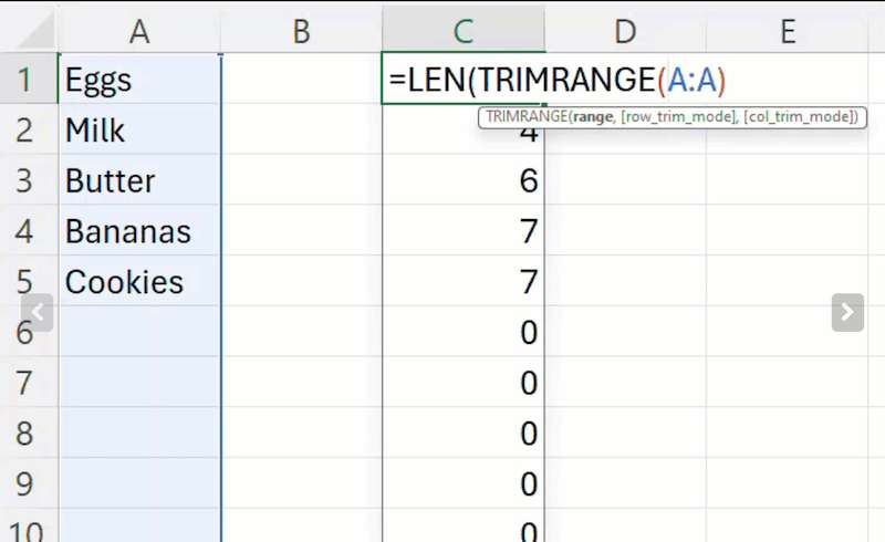
Using the TRIMRANGE function, you can write the word TRIMRANGE within the formula itself, such as =LEN(TRIMRANGE(A:A)). This specific formula will trim excess results in the range that no longer has any corresponding data in column A.
For instance, if you have data in Column A until A14 and you use the LEN and TRIMRANGE function in Column C, your spreadsheet will only show results until C14.
If you add data to A15, A16, and A17, it will also automatically show results in C15, C16 and C17.
So, the syntax when using TRIMRANGE function in your Excel is =TRIMRANGE(range,[trim_rows],[trim_cols]), whereas you indicate the range to be trimmed, which rows to be trimmed and which columns to be trimmed.
Wrapping Up
Cleaning your Excel spreadsheet will give you a presentable output while decluttering the space for unessential data. Hopefully TRIMRANGE can be useful for your next spreadsheet cleanup.