
We all know that rounding off numbers can help us solve mental equations faster. It is easier to solve 200 plus 500 than 248 plus 497. It helps when you buy things or want to know the value of something.
But, when you are dealing with accurate numbers, rounding off will not be as effective as creating mathematical decisions. Each number on the place values matters and can affect other numbers or the total.
Many users find it efficient to use Google Sheets when entering and organizing numbers in a worksheet. However, there are times when Google Sheets automatically rounds off the numbers. It is frustrating not to notice it and then realize the huge difference to your succeeding numbers.
When you do not want this to happen, you can stop Google Sheets from rounding your numbers. Follow the steps below to know how you can do it.
How to Tell Google Sheets to Stop Rounding your Numbers
Take note that Google Sheets follow the same mathematical rule when rounding off numbers. When the value is less than five, it retains the number on its left. When it is five to nine, it adds a number on its left.
To stop Google Sheets from rounding off your numbers, you will need to use the Truncate function. Using this function, it will show the decimal places without rounding off the number. All the values are retained even if you trim down your decimal places to two or add it up to five.
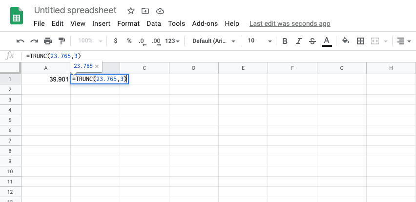
When using the Truncate function, you need to use this code: =TRUNC().
Inside the parenthesis should include the value of your number and the number of decimals, separated by a comma. For example, =TRUNC(23.765,3), where 23.765 is the value or amount that you want to show, and 3 is the number of decimal places.
Instead of the actual amount or value of the number, you can also use the cell location. For example, =TRUNC(C6,4), where C6 is the cell location of your number, and 4 is the number of decimal places.
Now, if you want to truncate the sum total of your number, add TRUNC before your Sum function. For example, =TRUNC(SUM(D2:D15,4).
Was the article helpful? Tell us in the comments below.
”Now, if you want to truncate the sum total of your number, add TRUNC before your Sum function. For example, =TRUNC(SUM(D2:D15,4).”
That functon is plain wrong, thanks for spreading misinformation.
Wrong/unhelpful.
“=TRUNC(11.99,2)” still told Google Sheets to display $12 instead of $11.99
Here’s how to stop the rounding:
1. Highlight/select the cell(s) in question.
2. Click “format” in the toolbar at the top.
3. Hover over/select “Number >”
4. Set it to “Currency ($1,000.12)”
Thanks! This was the fix.
So helpful! Thank you!
This “hack” does the exact opposite of what it claims.