
Organizing data is easier with Microsoft Excel. The spreadsheet tool allows you to manage data in each cell so you could edit them one at a time or all together. It saves you time and gives you a clean-looking and more professional document.
But, with a lot of data encoded in Excel, sometimes it is hard to find the information we want. Each cell looks similar to each other. We have to look twice to see what we are looking for.
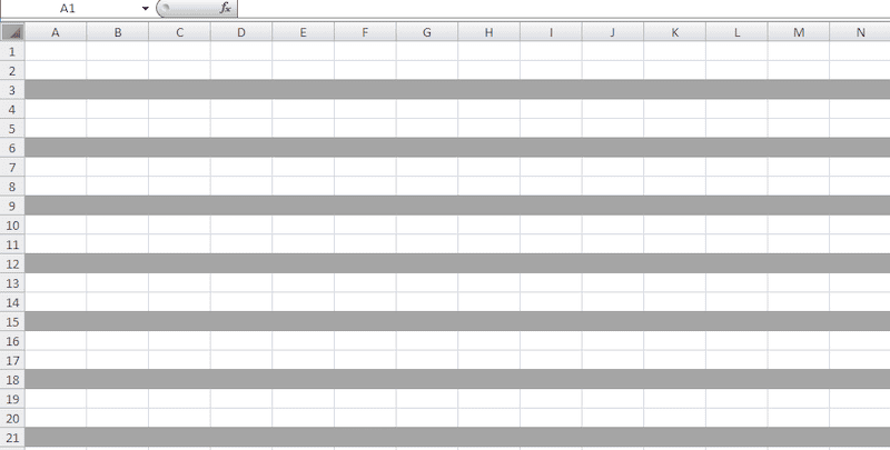
One way for us to find data more conveniently is to highlight every other row. That way, we don’t have to see things all alike and strain our eyes checking every row. Highlights or shade will allow you to identify each row and make each data more readable.
Ways to Shade or Highlight Every Other Row in Excel Worksheet
There are several ways on how you could make your Excel worksheet data readable, cleaner, and more organized. Check each method below and see which one works for your best. Follow the steps to know how to do it.
Method #1 – Creating Alternating Colors in Excel Table
You can edit the cell highlights by using the table feature in Microsoft Excel.
- First, highlight the rows that you want to edit.
- On the Home tab, look for the Styles option.
- Click the Format as Table button.
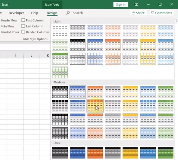
- Now, select the type of formatting you want to highlight each row. Available formats will give you alternating colors for highlight.
- Once you found the format you want to use, click to apply it to your cells.
- If there is nothing you like from the options, you can customize your table by clicking the New Table Style.
- Now, edit it based on how you want it.
Method #2 – Select Every Other Row in MS Excel
This method will take more time and effort to do. But, it will enable you to customize it. You can manually select the colors for each row.
- Select the row that you want to highlight by clicking the row number on the left.
- On the Home tab, go to the Font option.
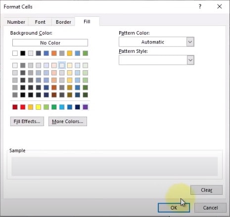
- Click the Fill Color button. It looks like a paint bucket icon.
- Click the color that you want. You can also find more colors by clicking the More Colors option.
- Do the same to all the rows that you want to highlight.
Method #3 – Using Conditional Formatting to Shade Alternate Rows in Excel
- To start, select all the rows that you want to highlight.
- Go to the Styles option on the Home tab.
- Click the Conditional Formatting button.
- Click New Rule.
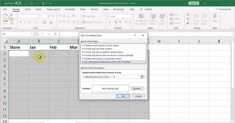
- Select a Rule Type.
- Under the Format values where this formula is true, enter =MOD(ROW(),2)=0,$A2<>””). If you want to alternate colors every three rows, change the number 2 to 3. You can change the formula numbers based on how you want the colors to appear on your spreadsheet.
- Click the Format button.
- Now, select the formatting.
- Click OK.
Did the article help you? Let us know in the comments below.